The Volatility Decay Example Most People Get Wrong
The usual volatility-decay example has a small problem: a 10% gain followed by a 10% loss does not get you back to even. I prefer to close that loop properly, because the corrected math is actually more useful.
This is not a technicality for its own sake. It separates the volatility drag every compounding investment experiences from the additional gap created when a leveraged ETF applies 2× or 3× exposure one day at a time.
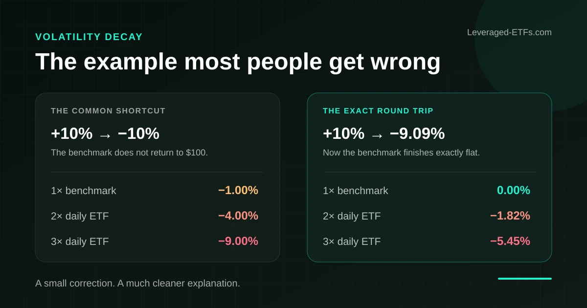
The familiar +10% / −10% example is not a round trip
Start with $100. A 10% gain takes the benchmark to $110. A 10% loss then removes $11—not the original $10—so the benchmark finishes at $99. The two percentage moves sum to zero, but the compounded return is −1%.
| Exposure | After +10% | After −10% | Two-day return |
|---|---|---|---|
| 1× benchmark | $110.00 | $99.00 | −1.00% |
| 2× daily ETF | $120.00 | $96.00 | −4.00% |
| 3× daily ETF | $130.00 | $91.00 | −9.00% |
There is nothing wrong with this example if it is labeled honestly. It demonstrates geometric compounding, and the leveraged results are striking. It just does not isolate leveraged ETF volatility decay because the benchmark itself has already lost money.
The corrected volatility decay example
To return from $110 to $100, the benchmark must fall by 10 divided by 110, or 9.0909%. Apply that exact decline and the benchmark closes the round trip at precisely $100.
| Exposure | After +10% | After −9.09% | Two-day return |
|---|---|---|---|
| 1× benchmark | $110.00 | $100.00 | 0.00% |
| 2× daily ETF | $120.00 | $98.18 | −1.82% |
| 3× daily ETF | $130.00 | $94.55 | −5.45% |
I prefer this version because there is nowhere for the effect to hide. The benchmark is flat, while the 2× ETF loses 1.82% and the 3× ETF loses 5.45%. Those values assume each fund delivers its daily objective perfectly and exclude fees, financing, and tracking differences.
For the product formula, more examples, and a calculator that repeats this round trip, use our complete guide to volatility decay in leveraged ETFs.
What daily resetting actually changes
A daily leveraged ETF normally targets a multiple of its benchmark's return for one trading day. After that day, the fund resets its exposure around a new value. The next return therefore acts on a different dollar base.
In the exact example, the 2× ETF does what it says: it gains 20% on day one and loses 18.18% on day two. The surprising multi-day result is not evidence that either daily return failed. It is the product of those returns.
The reset does not deduct a mysterious charge from the account. Actual funds have real costs, but volatility decay itself is a compounding result. Keeping those ideas separate makes the discussion far less slippery.
What this example proves
- A benchmark's start and end values are not enough to determine a daily leveraged ETF's return.
- Reversals can leave a negative compounding gap even when the benchmark finishes flat.
- The gap grows nonlinearly with leverage; the 3× loss is not merely 50% larger than the 2× loss.
- Percentage gains and losses are asymmetric because they apply to changing values.
What it absolutely does not prove
A tidy two-day round trip does not prove that leveraged ETFs inevitably lose value. When daily returns trend in the same direction, compounding can work in the investor's favor. Two consecutive benchmark gains of 5%, for example, produce 10.25% in the benchmark and 21% in a perfect 2× ETF—slightly more than twice the cumulative gain.
That favorable effect is the other side of the same mathematics. Our guide to leverage expansion walks through it without pretending that trends are guaranteed to continue.
The example also cannot answer whether a particular fund is suitable for a particular holding period. Direction, realized volatility, financing costs, fund expenses, tracking, taxes, and the investor's tolerance for severe drawdowns all matter.
A real market path is messier—and more useful
Once the two-day arithmetic is clear, I would stop stretching it into an investment conclusion. Real markets mix trends, reversals, calm stretches, and sudden shocks. A historical simulation is a better place to study how those pieces interacted over months or years.
Use the leveraged ETF backtesting tool to inspect a specific period, then read how the simulations account for leverage costs and real ETF data. The model is still not a forecast, but it is much closer to the question most investors are actually asking.
A necessary risk note
Leveraged ETFs are complex products that can experience substantial and sudden losses. Read the fund's daily investment objective and prospectus before investing. This article is educational and is not financial advice.
Sources and further reading
Try the exact example yourself
Change the leverage, upward move, and number of round trips to see how quickly the compounding gap changes.
Open the volatility decay calculator